How to remove duplicates in Google Sheets: A step-by-step guide

Google Sheets is a great spreadsheet application to create and edit files online while collaborating with others in real-time. Google sheet offers a host of features including editor-specific colour and history revision. In addition to this, the application is compatible with Microsoft Excel. Here, we will look at three methods, which have easy and simple steps to remove duplicates from Google Sheets. Also Read: What Is Seedream 4.0? The Google Gemini AI Nano Banana Rival By TikTok Parent Company

How to remove duplicates in Google Sheets using the ‘Remove Duplicates’ tool

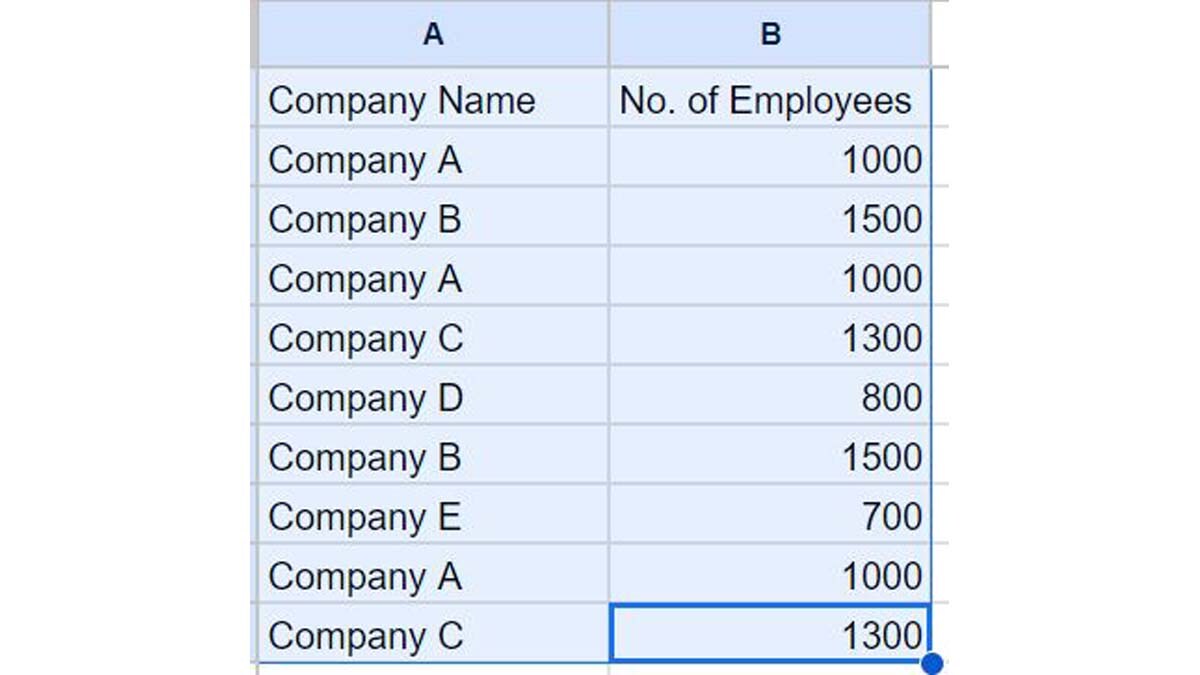
Step 1: Selected the dataset from where you want to remove the duplicates. Also Read: Gmail Introduces New 'Purchases' Tab Ahead Of Amazon Great Indian Festival And Flipkart Big Billion Days Sale: What Is It?

Also Read: How To Create Your 3D Figurine With Google Nano Banana AI Image Tool: Step-By-Step Guide With Prompt

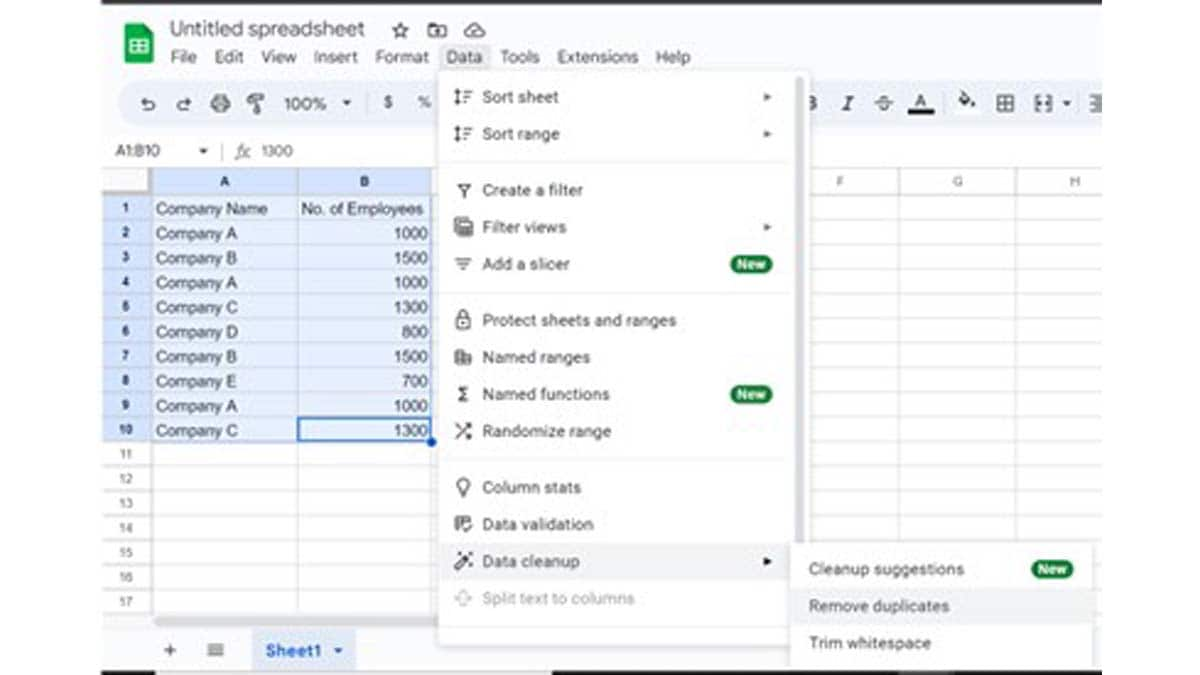
Step 2: Go to the Data option in the menu and click Data cleanup and then click on Remove duplicates. 

Step 3: In the Remove duplicates dialogue box, select Data has header row in case your data has a header row. 

Step 4: Under Columns to analyze select the columns that you want to analyse. If you select only one of the columns, the duplicates will get removed based on the data in that column only. 

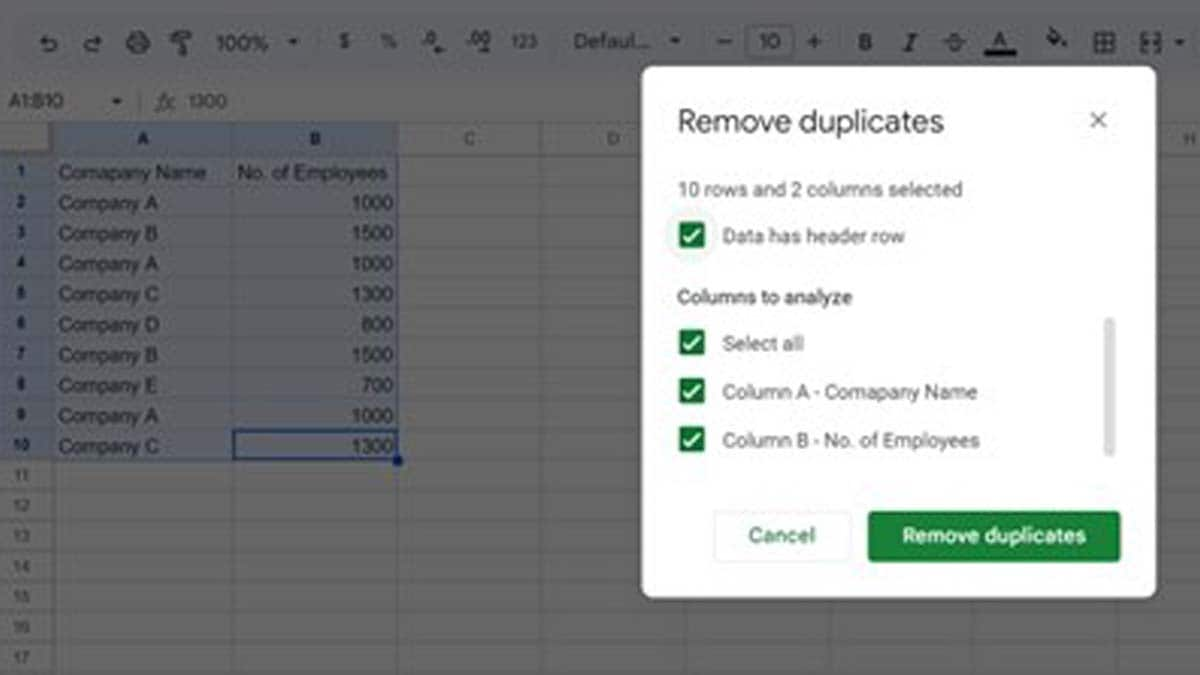
Step 5: Click on the Remove duplicates button.

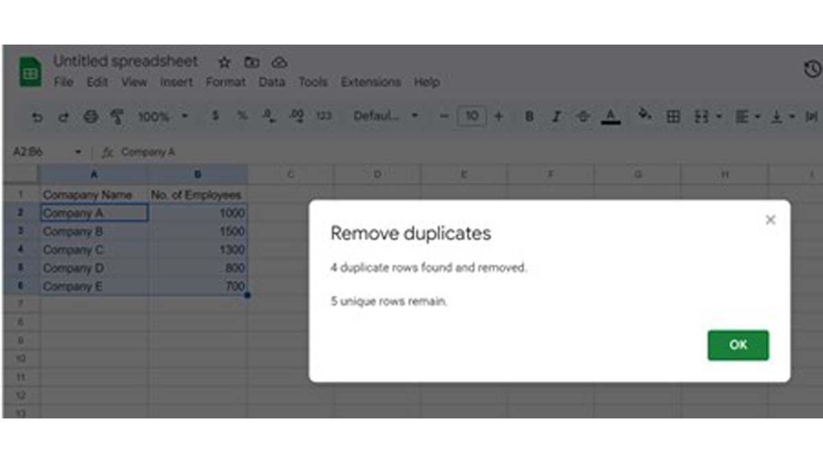
Step 6: On the prompt, click OK.

If you want to remove data from one column only, select data in that column and follow the above steps. Duplicate data will get removed without disturbing the data in other columns. 

How to remove duplicates in Google Sheets using the UNIQUE function

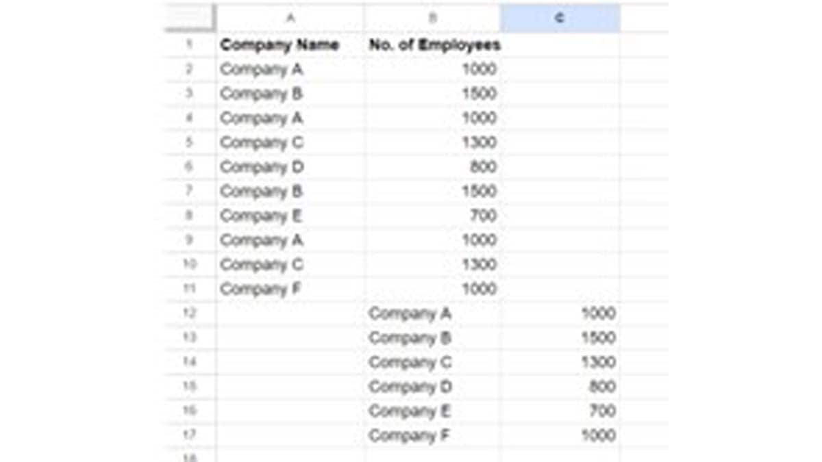
Step 1: Write ‘=UNIQUE(Column: Row)’ in any cell where you want your output. In the place of ‘Column’ put the first-row value of the dataset and in the place of ‘Row’ put last the last-row value of the dataset you want to analyse, as shown in the picture below.

Step 2: Press enter, and you will have your cleaned data set.

Please note the function will consider only those content as duplicates where an entire row content repeats. Further, if your data has extra space or leading or trailing space, the function will treat them as different. 

How to remove duplicates in Google Sheets using Conditional formatting 

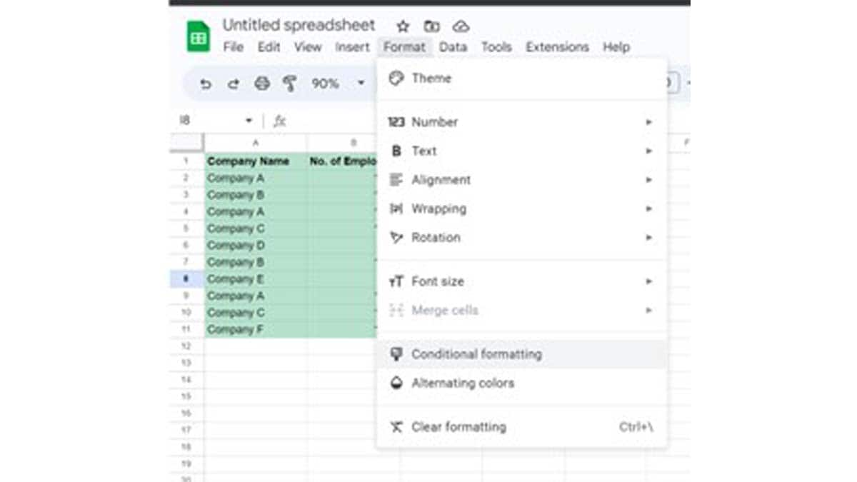
Step 1: Select the range of data from where you want to remove the duplicates. Leave the header column while selecting. 

Step 2: Go to Format and then Conditional formatting.

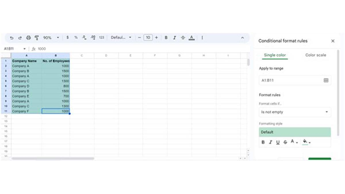
Step 3: In the Conditional format rules window, go to the Format rules and from the drop-down select Custom formula is.

Step 4: Input the formula =(COUNTIF($A$1:$A,$A1)>1)*(COUNTIF($B$1:$B,$B1)>1) and click Done.

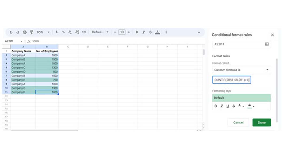
Duplicates in your data will be highlighted. You can change the highlight colour on the conditional format menu. Further, you can delete the duplicate value by using the backspace or delete row option.